Text mine in R using NLP techniques
In this article, I detail a method used to investigate a collection of text documents (corpus) and find the words (entities) that represent the collection of words in this corpus.
I will use an example where R, together with Natural Language Processing (NLP) techniques, is used to find the component of the system under test with the most issues found.
Operation Buggy
Say you are a tester and you are called in to help a DevOps team with their issue management system.
But the only thing you have been given are text documents made by the testers, which are exports of JIRA issues they reported.
They are large documents, and no one (including you) has time to manually read through them.
As a data scientist and QA expert, it’s your job to make sense of the data in the text documents.
What parts of the system were tested, and which system components had the most found issues? This is where Natural Language Processing (NLP) can enter to tackle the problem, and R, the statistical computing environment with different R packages, can be used to perform NLP methods on your data.
(Some packages include: tm, test reuse, openNLP, etc.) The choice of package depends on what you want to analyze with your data.
In this example, the immediate objective is to turn a large library of text into actionable data to:
- Find the issues with the highest risks (not the most buggy components of the system, because this component can also contain a lot of trivial issues).
- Fix the component of the system with the most issues.
To tackle the problem, we need statistics.
By using the statistical programming language R, we can make statistical algorithms to find the most buggy component of the system under test.
Retrieval of the data
First, we have to retrieve and preprocess the files to enable the search for the most buggy component.
what R packages do we actually need?
These are mentioned in Table 1, including their functions.
 Table 1: R packages used
The functions of these R packages will be explained when the R packages are addressed.
Before you start to build the algorithm in R, you first have to install and load the libraries of the R packages.
After installation, every R script first starts with addressing the R libraries as shown below.
library(tm)
library(SnowballC)
library(topicmodels)
You can start with retrieving the dataset (or corpus for NLP).
For this experiment, we saved three text files with bug reports from three testers in a separate directory, also being our working directory (use setwd(“directory”) to set the working directory).
#set working directory (modify path as needed)
setwd(directory)
You can load the files from this directory in the corpus:
#load files into corpus
#get listing of .txt files in directory
filenames <- list.files(getwd(),pattern="*.txt") #getwd() represents working directory
Read the files into a character vector, which is a basic data structure and can be read by R.
#read files into a character vector
files <- lapply(filenames,readLines)
We now have to create a corpus from the vector.
#create corpus from vector
articles.corpus <- Corpus(VectorSource(files))
Table 1: R packages used
The functions of these R packages will be explained when the R packages are addressed.
Before you start to build the algorithm in R, you first have to install and load the libraries of the R packages.
After installation, every R script first starts with addressing the R libraries as shown below.
library(tm)
library(SnowballC)
library(topicmodels)
You can start with retrieving the dataset (or corpus for NLP).
For this experiment, we saved three text files with bug reports from three testers in a separate directory, also being our working directory (use setwd(“directory”) to set the working directory).
#set working directory (modify path as needed)
setwd(directory)
You can load the files from this directory in the corpus:
#load files into corpus
#get listing of .txt files in directory
filenames <- list.files(getwd(),pattern="*.txt") #getwd() represents working directory
Read the files into a character vector, which is a basic data structure and can be read by R.
#read files into a character vector
files <- lapply(filenames,readLines)
We now have to create a corpus from the vector.
#create corpus from vector
articles.corpus <- Corpus(VectorSource(files))
Preprocessing the data
Next, we need to preprocess the text to convert it into a format that can be processed for extracting information.
An essential aspect involves the reduction of the size of the feature space before analyzing the text, i.e.
normalization.
(Several preprocessing methods are available, such as case-folding, stop word removal, stemming, lemmatization, contraction simplification etc.) What preprocessing method is necessary depends on the data we retrieve, and the kind of analysis to be performed.
Here,we use case-folding and stemming.
Case-folding to match all possible instances of a word (Auto and auto, for instance).
Stemming is the process of reducing the modified or derived words to their root form.
This way, we also match the resulting root forms.
# make each letter lowercase
articles.corpus <- tm_map(articles.corpus, tolower)
#stemming
articles.corpus <- tm_map(articles.corpus, stemDocument);
Create the DTM
The next step is to create a document-term matrix (DTM).
This is critical, because to interpret and analyze the text files, they must ultimately be converted into a document-term matrix.
The DTM holds the number of term occurrences per document.
The rows in a DTM represent the documents, and each term in a document is represented as a column.
We’ll also remove the low-frequency words (or sparse terms) after converting the corpus into the DTM.
articleDtm <- DocumentTermMatrix(articles.corpus, control = list(minWordLength = 3));
articleDtm2 <- removeSparseTerms(articleDtm, sparse=0.98)
Topic modeling
We are now ready to find the words in the corpus that represent the collection of words used in the corpus: the essentials.
This is also called topic modeling.
The topic modeling technique we will use here is latent Dirichlet allocation (LDA).
The purpose of LDA is to learn the representation of a fixed number of topics, and given this number of topics, learn the topic distribution that each document in a collection of documents has.
Explaining LDA goes far beyond the scope of this article.
For now, just follow the code as written below.
#LDA
k = 5;
SEED = 1234;
article.lda <- LDA(articleDtm2, k, method="Gibbs", control=list(seed = SEED))
lda.topics <- as.matrix(topics(article.lda))
lda.topics
lda.terms <- terms(article.lda)
If you now run the full code in R as explained above, you will calculate the essentials, the words in the corpus that represent the collection of words used in the corpus.
For this experiment, the results were:
> lda.terms
Topic 1 Topic 2 Topic 3 Topic 4 Topic 5
"theo" "customers" "angela" "crm" "paul"
Topics 1 and 3 can be explained: theo and angela are testers.
Topic 5 is also easily explained: paul is a fixer.
Topic 4, crm, is the system under test, so it’s not surprising it shows up as a term in the LDA, because it is mentioned in every issue by every tester.
Now, we still have topic 2: customers.
Customers is a component of the system under test: crm.
Customers is most mentioned as a component in the issues found by all the testers involved.
Finally, we have found our most buggy component.
Wrap-up
This article described a method we can use to investigate a collection of text documents (corpus) and find the words that represent the collection of words in this corpus.
For this article’s example, R (together with NLP techniques) was used to find the component of the system under test with the most issues found.
R code
library(tm)
library(SnowballC)
library(topicmodels)
# TEXT RETRIEVAL
#set working directory (modify path as needed)
ld
#load files into corpus
#get listing of .txt files in directory
filenames <- list.files(getwd(),pattern="*.txt")
#read files into a character vector
files <- lapply(filenames,readLines)
#create corpus from vector
articles.corpus <- Corpus(VectorSource(files))
# TEXT PROCESSING
# make each letter lowercase
articles.corpus <- tm_map(articles.corpus, tolower)
# stemming
articles.corpus <- tm_map(articles.corpus, stemDocument);
# Ceate the Document Term Matrix (DTM)
articleDtm <- DocumentTermMatrix(articles.corpus, control = list(minWordLength = 3));
articleDtm2 <- removeSparseTerms(articleDtm, sparse=0.98)
# TOP MODELING
k = 5;
SEED = 1234;
article.lda <- LDA(articleDtm2, k, method="Gibbs", control=list(seed = SEED))
lda.topics <- as.matrix(topics(article.lda))
lda.topics
lda.terms <- terms(article.lda)
lda.terms
7 Excellent R Natural Language Processing Tools
Python and R stand toe-to-toe in data science.
But in the field of NLP, Python stands very tall.
The Natural Language Toolkit (NLTK) for Python is an awesome library and set of corpuses.
However, R offers competent libraries for natural language processing.
Many of the techniques such as word and sentence tokenization, n-gram creation, and named entity recognition are easily performed in R.
Start with NLP, offering basic classes and methods.
Then take a gander at openNLP which provides an interface to the Apache OpenNLP tools.
Speaking of interfaces, there’s also RWeka, an R interface to Weka.
But there’s some excellent R packages if you look further afield.
Here’s our recommendations.
 Let’s explore the R based NLP tools at hand.
For each title we have compiled its own portal page, a full description with an in-depth analysis of its features, together with links to relevant resources.
Let’s explore the R based NLP tools at hand.
For each title we have compiled its own portal page, a full description with an in-depth analysis of its features, together with links to relevant resources.
| R Natural Language Processing Tools |
| tidytext | Text mining using dplyr, ggplot2, and other tidy tools |
| text2vec | Framework with API for text analysis and natural language processing |
| quanteda | R package for Quantitative Analysis of Textual Data |
| wordcloud | Create attractive word clouds |
| tm | Text Mining Infrastructure in R |
| Word Vectors | Build and explore embedding models |
| UDPipe | Tokenization, Tagging, Lemmatization and Dependency Parsing |
Topic Modeling and Music Classification
In this tutorial, you will build four models using Latent Dirichlet Allocation (LDA) and K-Means clustering machine learning algorithms to build your own music recommendation system!
This is part Two-B of a three-part tutorial series in which you will continue to use R to perform a variety of analytic tasks on a case study of musical lyrics by the legendary artist Prince, as well as other artists and authors.
The three tutorials cover the following:
Imagine you are a Data Scientist working for NASA.
You are asked to monitor two spacecraft intended for lunar orbits, which will study the moon's interactions with the sun.
As with any spacecraft, there can be problems that are captured during test or post-launch.
These anomalies are documented in natural language into nearly 20,000 problem reports.
Your job is to identify the most popular topics and trending themes in the corpus of reports and provide prescriptive analysis results to the engineers and program directors, thus impacting the future of space exploration.
This is an example of a real-life scenario and should give you an idea of the power you'll have at your fingertips after learning how to use cutting-edge techniques, such as topic modeling with machine learning, Natural Language Processing (NLP) and R programming.
Luckily, you don't have to work for NASA to do something just as innovative.
In this tutorial, your mission, should you choose to accept it, is to learn about topic modeling and how to build a simple recommendation (a.k.a recommender) system based on musical lyrics and nonfiction books.
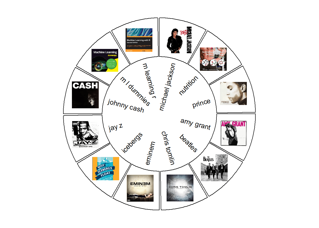
Just For Fun!
This has nothing to do with topic modeling, but just for fun, use a great package called circlize, introduced in a previous tutorial, to fire up those photoreceptors and enjoy this circle diagram of all the sources you'll use in this tutorial.
library(jpeg)
library(circlize) #you'll use this package later
#read in the list of jpg files of album/book covers
CELL_META$sector.index,
CELL_META$sector.index, facing = "clockwise", niceFacing = TRUE,
adj = c(1, 0.5), cex = 0.9)
circos.raster(image, CELL_META$xcenter, CELL_META$ycenter, width = "1.5cm",
facing = "downward")
}, bg.border = 1, track.height = .4)
 Structure
In previous tutorials, you studied the content of Prince's lyrics using word frequency, the tf-idf statistic, and sentiment analysis.
You can get deeper insight into lyrics and other text by using the concept of topic modeling.
In this tutorial, you will build four models using Latent Dirichlet Allocation (LDA) and K-Means clustering machine learning algorithms.
I will explain the algorithms later in the tutorial.
Model One utilizes text from Prince's lyrics combined with two nonfiction books.
The objective of this model is to give you a simple example of using LDA, an unsupervised algorithm, to generate collections of words that together suggest themes.
These themes are unlabeled and require human interpretation.
Once you have identified a predefined number of themes, you will then take the results of your model and classify each song or book page into each category.
A song may contain all the topics you've generated but may fit more cleanly into one over another.
This is referred to as document classification, but since you know the writer of the document, you are essentially classifying writers into thematic groupings.
Model Two uses the Model One dataset and gives a quick glance into generating themes using a different algorithm, k-means, and how it may not be the best choice for topic modeling.
Once again using LDA, Model Three utilizes a larger dataset with multiple artists from different genres and more book authors.
When you classify the majority of documents from an author/artist into their most likely topic, you have created the ability to group writers with similar thematic compositions.
With a solid model, you should see similar genres appear in the same topic grouping.
For example, rap artists would appear in one topic, and two books on a similar subject should appear together in a different topic.
Thus, you could potentially recommend similar writers! Obviously, the writers and their genre are labeled, but the topics are not, and are therefore unsupervised.
Model Four uses LDA only on Prince's lyrics.
This time you'll use an annotated dataset generated outside of this tutorial that has each word tagged as a part of speech (i.e.
noun, verb, etc.) as well as the root form (lemmatized) of the word.
You will also examine how a topic changes over time.
Structure
In previous tutorials, you studied the content of Prince's lyrics using word frequency, the tf-idf statistic, and sentiment analysis.
You can get deeper insight into lyrics and other text by using the concept of topic modeling.
In this tutorial, you will build four models using Latent Dirichlet Allocation (LDA) and K-Means clustering machine learning algorithms.
I will explain the algorithms later in the tutorial.
Model One utilizes text from Prince's lyrics combined with two nonfiction books.
The objective of this model is to give you a simple example of using LDA, an unsupervised algorithm, to generate collections of words that together suggest themes.
These themes are unlabeled and require human interpretation.
Once you have identified a predefined number of themes, you will then take the results of your model and classify each song or book page into each category.
A song may contain all the topics you've generated but may fit more cleanly into one over another.
This is referred to as document classification, but since you know the writer of the document, you are essentially classifying writers into thematic groupings.
Model Two uses the Model One dataset and gives a quick glance into generating themes using a different algorithm, k-means, and how it may not be the best choice for topic modeling.
Once again using LDA, Model Three utilizes a larger dataset with multiple artists from different genres and more book authors.
When you classify the majority of documents from an author/artist into their most likely topic, you have created the ability to group writers with similar thematic compositions.
With a solid model, you should see similar genres appear in the same topic grouping.
For example, rap artists would appear in one topic, and two books on a similar subject should appear together in a different topic.
Thus, you could potentially recommend similar writers! Obviously, the writers and their genre are labeled, but the topics are not, and are therefore unsupervised.
Model Four uses LDA only on Prince's lyrics.
This time you'll use an annotated dataset generated outside of this tutorial that has each word tagged as a part of speech (i.e.
noun, verb, etc.) as well as the root form (lemmatized) of the word.
You will also examine how a topic changes over time.
Introduction
NLP and Machine Learning are subfields of Artificial Intelligence.
There have been recent attempts to use AI for songwriting.
That's not the goal of this tutorial, but it's an example of how AI can be used as art.
After all, the first three letters are A-R-T! Just for a moment, compare AI to songwriting: you can easily follow a pattern and create a structure (verse, chorus, verse, etc.), but what makes a song great is when the writer injects creativity into the process.
In this tutorial, you'll need to exercise your technical skills to build models, but you'll also need to invoke your artistic creativity and develop the ability to interpret and explain your results.
Consider this: If topic modeling is an art, then lyrics are the code, songwriting is the algo-rhythm, and the song is the model! What's your analogy?
Typical recommendation systems are not based entirely on text.
For example, Netflix can recommend movies based on previous choices and associated metadata.
Pandora has a different approach and relies on a Music Genome consisting of 400 musical attributes, including melody, rhythm, composition and lyric summaries; however, this genome development began in the year 2000 and took five years and 30 experts in music theory to complete.
There are plenty of research papers addressing movie recommendations based on plot summaries.
Examples of music recommendation systems based on actual lyrical content are harder to find.
Want to give it a try?
- Prerequisites
Part Two-B of this tutorial series requires a basic understanding of tidy data - specifically packages such as dplyr and ggplot2.
Practice with text mining using tidytext is also recommended, as it was covered in the previous tutorials.
You'll also need to be familiar with R functions, as you will utilize a few to reuse your code for each model.
In order to focus on capturing insights, I have included code that is designed to be used on your own dataset, but detailed explanation may require further investigation on your part.
- Prepare Your Questions
What can you do with topic modeling? Maybe there are documents that contain critical information to your business that you could mine.
Maybe you could scrape data from Twitter and find out what people are saying about your company's products.
Maybe you could build your own classification system to send certain documents to the right departments for analysis.
There is a world of possibilities that you can explore! Go for it!
- Why is Topic Modeling Useful?
Here are several applications of topic modeling:
- Document summaries: Use topic models to understand and summarize scientific articles enabling faster research and development.
The same applies to historical documents, newspapers, blogs, and even fiction.
- Text classification: Topic modeling can improve classification by grouping similar words together in topics rather than using each word as an individual feature.
- Recommendation Systems: Using probabilities based on similarity, you can build recommendation systems.
You could recommend articles for readers with a topic structure similar to articles they have already read.
- Do you have other ideas?
Prep Work
- Libraries and Functions
The only new packages in this tutorial that are not in Part One or Part Two-A are topicmodels, tm, and plotly.
You'll use the LDA() function from topicmodels which allows models to learn to distinguish between different documents.
The tm package is for text mining, and you just use the inspect() function once to see the inside of a document-term matrix, which I'll explain later.
You'll only use plotly once to create an interactive version of a ggplot2 graph.
library(tidytext) #text mining, unnesting
library(topicmodels) #the LDA algorithm
library(tidyr) #gather()
#customize the text tables for consistency using HTML formatting
my_kable_styling <- function(dat, caption) {
kable(dat, "html", escape = FALSE, caption = caption) %>%
kable_styling(bootstrap_options = c("striped", "condensed", "bordered"),
full_width = FALSE)
}
word_chart <- function(data, input, title) {
data %>%
#set y = 1 to just plot one variable and use word as the label
ggplot(aes(as.factor(row), 1, label = input, fill = factor(topic) )) +
#you want the words, not the points
geom_point(color = "transparent") +
#make sure the labels don't overlap
geom_label_repel(nudge_x = .2,
direction = "y",
box.padding = 0.1,
segment.color = "transparent",
size = 3) +
facet_grid(~topic) +
theme_lyrics() +
theme(axis.text.y = element_blank(), axis.text.x = element_blank(),
#axis.title.x = element_text(size = 9),
panel.grid = element_blank(), panel.background = element_blank(),
panel.border = element_rect("lightgray", fill = NA),
strip.text.x = element_text(size = 9)) +
labs(x = NULL, y = NULL, title = title) +
#xlab(NULL) + ylab(NULL) +
#ggtitle(title) +
coord_flip()
}
- Music and Books
In order to really see the power of topic modeling and classification, you'll not
- Get The Data
In order to focus on modeling, I performed data conditioning outside of this tutorial and have provided you with all the data you need in these three files below with the following conditioning already applied:
- scraped the web for lyrics of eight artists
- used the
pdf_text() function from the pdftools package to collect the content of four books (each page represents a distinct document)
- cleaned all the data, removed stop words, and created the tidy versions using the
tidytext package described in Part One
- combined and balanced the data such that each writer (source) has the same number of words
You will have three distinct datasets to work within this tutorial:
three_sources_tidy_balanced: contains Prince lyrics and two booksall_sources_tidy_balanced: contains lyrics from eight artists and four booksprince_tidy: contains only Prince lyrics
I've also included an annotated dataset of Prince's lyrics as well.
I will explain what is meant by annotated when you get to Model Four.
#Get Tidy Prince Dataset and Balanced Tidy Dataset of All Sources and 3 Sources
- During initialization, each word is assigned to a random topic
- The algorithm goes through each word iteratively and reassigns the word to a topic with the following considerations:
- the probability the word belongs to a topic
- the probability the document will be generated by a topic
The concept behind the LDA topic model is that words belonging to a topic appear together in documents.
It tries to model each document as a mixture of topics and each topic as a mixture of words.
(You may see this referred to as a mixed-membership model.) You can then use the probability that a document belongs to a particular topic to classify it accordingly.
In your case, since you know the writer of the document from the original data, you can then recommend an artist/author based on similar topic structures.
Now it's time to take a look at an example.
Model One: LDA for Three Writers
- Examine The Data
For this model, you will use the dataset with a combination of three distinct writers (i.e.
sources) and look for hidden topics.
In order to help you understand the power of topic modeling, these three chosen sources are very different and intuitively you know they cover three different topics.
As a result, you'll tell your model to create three topics and see how smart it is.
First you want to examine your dataset using your my_kable_styling() function along with color_bar() and color_tile() from the formattable package.
#group the dataset by writer (source) and count the words
three_sources_tidy_balanced %>%
group_by(source) %>%
tidytext/versions/0.1.3/topics/cast_tdm_" target="_blank">cast_dtm() function where document is the name of the field with the document name and word is the name of the field with the term.
There are other parameters you could pass, but these two are required.
three_sources_dtm_balanced <- three_sources_tidy_balanced %>%
#get word count per document to pass to cast_dtm
A short technical explanation of GIBBS sampling is that it performs a random walk that starts at some point which you can initialize (you'll just use the default of 0) and at each step moves plus or minus one with equal probability.
Read a detailed description here if you are interested in the details.
Note: I have glossed over the details of the LDA algorithm.
Although you don't need to understand the statistical theory in order to use it, I would suggest that you read this document by Ethen Liu which provides a solid explanation.
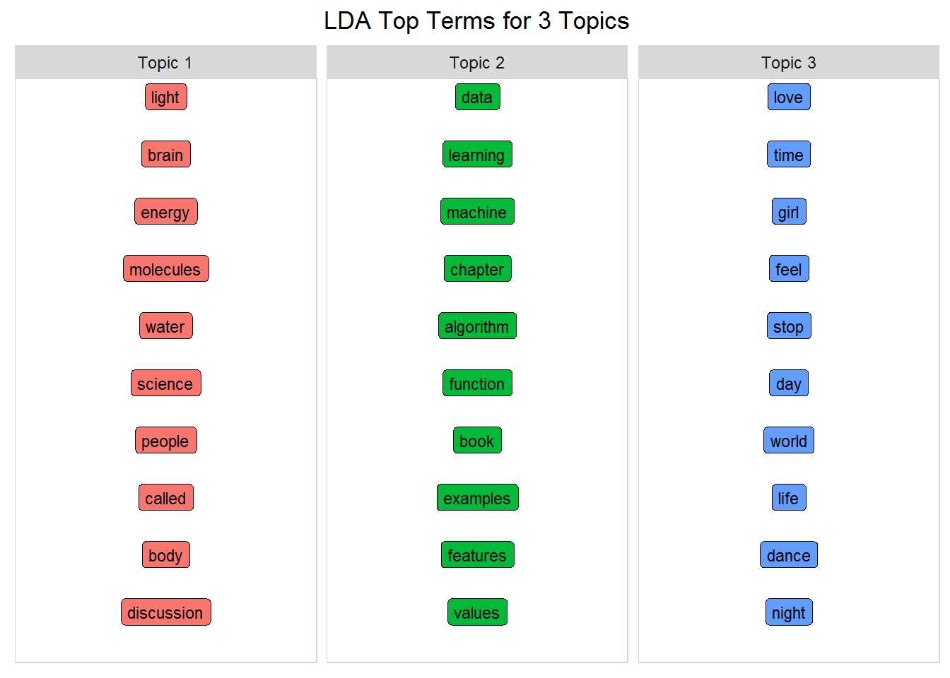
k <- 3 #number of topics
seed = 1234 #necessary for reproducibility
num_words <- 10 #number of words to visualize
#create function that accepts the lda model and num word to display
top_terms_per_topic <- function(lda_model, num_words) {
mutate(topic = paste("Topic", topic, sep = " "))
#create a title to pass to word_chart
title <- paste("LDA Top Terms for", k, "Topics")
#call the word_chart function you built in prep work
word_chart(top_terms, top_terms$term, title)
}
#call the function you just built!
top_terms_per_topic(lda, num_words)
#this time use gamma to look at the prob a doc is in a topic
#just look at the Prince song 1999 as an example
tidy(lda, matrix = "gamma") %>% filter(document == "1999")
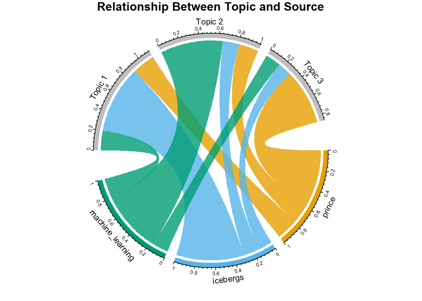
the circlize package.
All you'll ever need to know about the package is covered in this book by Zuguang Gu.)
#using tidy with gamma gets document probabilities into topic
#but you only have document, topic and gamma
source_topic_relationship <- tidy(lda, matrix = "gamma") %>%
circos.clear() #very important! Reset the circular layout parameters
#assign colors to the outside bars around the circle
grid.col = c("prince" = my_colors[1],
"icebergs" = my_colors[2],
"machine_learning" = my_colors[3],
"Topic 1" = "grey", "Topic 2" = "grey", "Topic 3" = "grey")
# set the global parameters for the circular layout.
Specifically the gap size (15)
#this also determines that topic goes on top half and source on bottom half
circos.par(gap.after = c(rep(5, length(unique(source_topic_relationship[[1]])) - 1), 15,
rep(5, length(unique(source_topic_relationship[[2]])) - 1), 15))
#main function that draws the diagram.
transparancy goes from 0-1
chordDiagram(source_topic_relationship, grid.col = grid.col, transparency = .2)
title("Relationship Between Topic and Source")
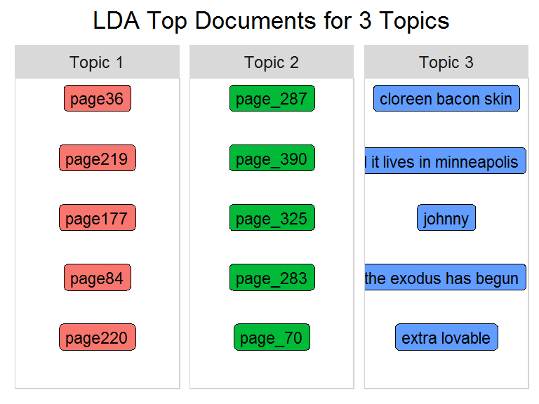
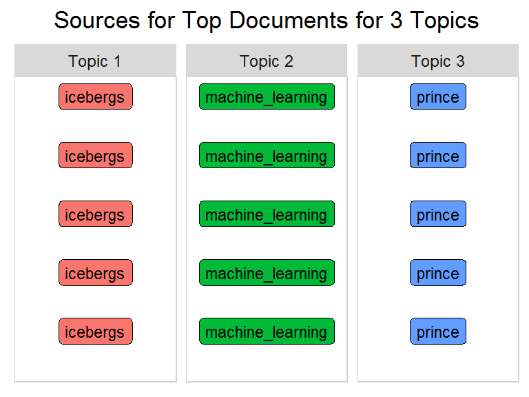
-- Top Documents Per Topic
Now look at the individual document level and view the top documents per topic.
number_of_documents = 5 #number of top docs to view
title <- paste("LDA Top Documents for", k, "Topics")
title <- paste("LDA Top Documents for", k, "Topics")
word_chart(top_documents, top_documents$document, title)
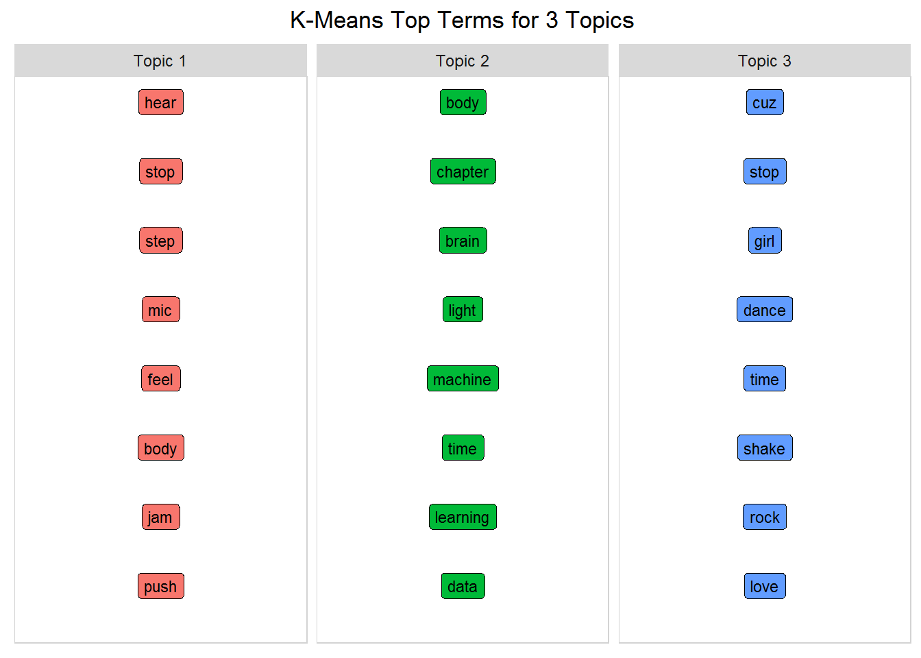
 based on a similarity measure.
It transforms documents to a numeric vector with weights assigned to words per document (similar to tf-idf).
Each document will show up in exactly one cluster.
This is called hard clustering.
The output is a set of clusters along with their documents.
In contrast, LDA is a fuzzy (soft) clustering technique where a data point can belong to more than one cluster.
So conceptually, when applied to natural language, LDA should give more realistic results than k-means for topic assignment, given that text usually entails more than one topic.
Build your model now, examine the k-means object, and see if your assumption holds true.
based on a similarity measure.
It transforms documents to a numeric vector with weights assigned to words per document (similar to tf-idf).
Each document will show up in exactly one cluster.
This is called hard clustering.
The output is a set of clusters along with their documents.
In contrast, LDA is a fuzzy (soft) clustering technique where a data point can belong to more than one cluster.
So conceptually, when applied to natural language, LDA should give more realistic results than k-means for topic assignment, given that text usually entails more than one topic.
Build your model now, examine the k-means object, and see if your assumption holds true.
- Set Variables and Fit The Model
#use the same three sources you started with
source_dtm <- three_sources_dtm_balanced
source_tidy <- three_sources_tidy_balanced
The structure of the k-means object reveals two important pieces of information: clusters and centers.
You can use the format below to see the contents of each variable for the song 1999 and the word <
kmeans_top_terms <- kmeans_top_terms %>%
group_by(topic) %>%
mutate(row = row_number()) %>% #needed by word_chart()
ungroup()
title <- paste("K-Means Top Terms for", k, "Topics")
word_chart(kmeans_top_terms, kmeans_top_terms$term, title)
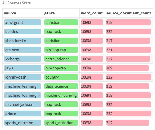
 sources/writers covering multiple genres.
The dataset is already balanced with a similar number of documents and words per writer.
Here is an overview of the data:
sources/writers covering multiple genres.
The dataset is already balanced with a similar number of documents and words per writer.
Here is an overview of the data:
- Examine The Data
all_sources_tidy_balanced %>%
group_by(source) %>%
#get the word count and doc count per source
 Don't forget about the mixed-membership concept and that these topics are not meant to be completely disjoint, but I was amazed to see the results as discrete as you see here.
Just as a side note: the LDA algorithm takes more parameters than you used and thus you can tune your model to be even stronger.
This next part is really exciting.
How can you make it easier to see what these topics are about? In most cases, it's tough to interpret, but with the right dataset, your model can perform well.
If your model can determine which documents are more likely to fall into each topic, you can begin to group writers together.
And since in your case you know the genre of a writer, you can validate your results - to a certain extent! The first step is to classify each document.
Don't forget about the mixed-membership concept and that these topics are not meant to be completely disjoint, but I was amazed to see the results as discrete as you see here.
Just as a side note: the LDA algorithm takes more parameters than you used and thus you can tune your model to be even stronger.
This next part is really exciting.
How can you make it easier to see what these topics are about? In most cases, it's tough to interpret, but with the right dataset, your model can perform well.
If your model can determine which documents are more likely to fall into each topic, you can begin to group writers together.
And since in your case you know the genre of a writer, you can validate your results - to a certain extent! The first step is to classify each document.
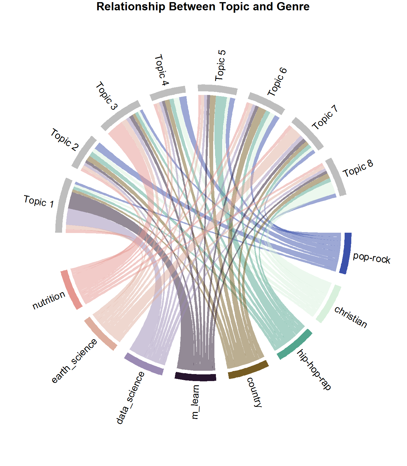
- Classify Documents
-- Chord Diagram
As a reminder, each document contains multiple topics, but at different percentages represented by the gamma value.
Some documents fit some topics better than others.
This plot shows the average gamma value of documents from each source for each topic.
This is the same approach you used above with three writers, except this time you'll look at the genre field.
It is a fantastic way of showing the relationship between the genre of the writers and the topics.
source_topic_relationship <- tidy(lda, matrix = "gamma") %>%
#join to the tidy form to get the genre field
grid.col = c("Topic 1" = "grey", "Topic 2" = "grey", "Topic 3" = "grey",
"Topic 4" = "grey", "Topic 5" = "grey", "Topic 6" = "grey",
"Topic 7" = "grey", "Topic 8" = "grey")
#set the gap size between top and bottom halves set gap size to 15
circos.par(gap.after = c(rep(5, length(unique(source_topic_relationship[[1]])) - 1), 15,
rep(5, length(unique(source_topic_relationship[[2]])) - 1), 15))
chordDiagram(source_topic_relationship, grid.col = grid.col, annotationTrack = "grid",
preAllocateTracks = list(track.height = max(strwidth(unlist(dimnames(source_topic_relationship))))))
#go back to the first track and customize sector labels
#use niceFacing to pivot the label names to be perpendicular
circos.track(track.index = 1, panel.fun = function(x, y) {
circos.text(CELL_META$xcenter, CELL_META$ylim[1], CELL_META$sector.index,
facing = "clockwise", niceFacing = TRUE, adj = c(0, 0.5))
}, bg.border = NA) # here set bg.border to NA is important
title("Relationship Between Topic and Genre")
 systems but could be combined with metadata such as rhythm, instrumentation, tempo, etc.., for a better listening experience.
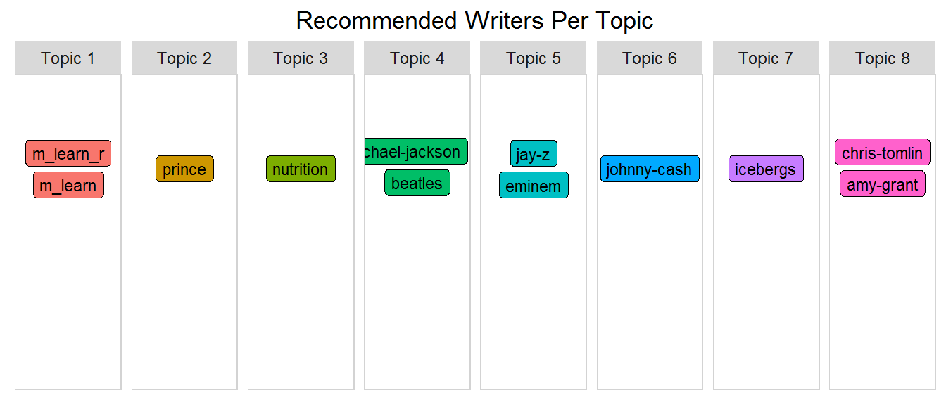
- Recommend Similar Writers
Now that you can see the relationship between documents and topics, group by source (i.e.
writer) and topic and get the sum of gamma values per group.
Then select the writer with the highest topic_sum for each topic using top_n(1).
Since you'll want to do the same thing for genre as you're doing here with writer, create a function called top_items_per_topic() and pass source as the type.
This way you'll be able to call it again when you classify documents by genre.
This is the critical moment where you actually map the writer to a specific topic.
What do you expect will happen?
#this function can be used to show genre and source via passing the "type"
top_items_per_topic <- function(lda_model, source_tidy, type) {
ungroup() %>%
#type will be either source or genre
group_by(source, genre ) %>%
#get the highest topic_sum per type
top_n(1, topic_sum) %>%
mutate(row = row_number()) %>%
mutate(label = ifelse(type == "source", source, genre),
title = ifelse(type == "source", "Recommended Writers Per Topic",
"Genres Per Topic")) %>%
ungroup() %>%
#re-label topics
mutate(topic = paste("Topic", topic, sep = " ")) %>%
select(label, topic, title)
#slightly different format from word_chart input, so use this version
document_lda_gamma %>%
#use 1, 1, and label to use words without numeric values
ggplot(aes(1, 1, label = label, fill = factor(topic) )) +
#you want the words, not the points
geom_point(color = "transparent") +
#make sure the labels don't overlap
geom_label_repel(nudge_x = .2,
direction = "y",
box.padding = 0.1,
segment.color = "transparent",
size = 3) +
facet_grid(~topic) +
theme_lyrics() +
theme(axis.text.y = element_blank(), axis.text.x = element_blank(),
axis.title.y = element_text(size = 4),
panel.grid = element_blank(), panel.background = element_blank(),
panel.border = element_rect("lightgray", fill = NA),
strip.text.x = element_text(size = 9)) +
xlab(NULL) + ylab(NULL) +
ggtitle(document_lda_gamma$title) +
coord_flip()
}
top_items_per_topic(lda, source_tidy, "source")
 be more mixed and less disjoint.
This makes interpretation a very critical step.
Instead of using the raw data from Prince's lyrics, you will use a slightly modified version as described below.
be more mixed and less disjoint.
This makes interpretation a very critical step.
Instead of using the raw data from Prince's lyrics, you will use a slightly modified version as described below.
- Use NLP To Improve Model
Previously you have used words as they appear in the text.
But now you'll use an annotated form of the data resulting from a powerful NLP package called cleanNLP.
This package is a tidy data model for Natural Language Processing that provides annotation tasks such as tokenization, part of speech tagging, named entity recognition, entity linking, sentiment analysis, and many others.
This exercise was performed outside of this tutorial, but I have provided all you'll need for topic modeling.
- Examine NLP Output
In the annotated dataset, there is one row for every word in the corpus of Prince's lyrics with important information about each word.
Take a closer look at the tokenized annotation object by examining the field names.
#read in the provided annotated dataset
prince_annotated <- read.csv("prince_data_annotated.csv")
#look at the fields provided in the dataset
t covered in Part One is another method you may consider for removing common words.)
- Set Variables Using NLP
source_tidy <- prince_annotated %>%
select(document = id, word, lemma, upos) %>%
filter(upos == "NOUN") %>% #choose only the nouns
It seems that your Topic 1 is about people and family; Topic 7 is about music, dance and party; and Topic 4 is about self, society, and religion.
This requires very subjective interpretation.
In a business context, this step is best performed by a subject matter expert who may have an idea of what to expect.
Now you can see why NLP is truly the intersection of artificial intelligence and computational linguistics!
Try running this with a different number of topics, or with just verbs, or using the raw word versus the lemmatized form, or with a different number of top words and see what insights you can derive.
There are new methods to help you determine the number of topics: see the concept of perplexity here, or the ldatuning package here.
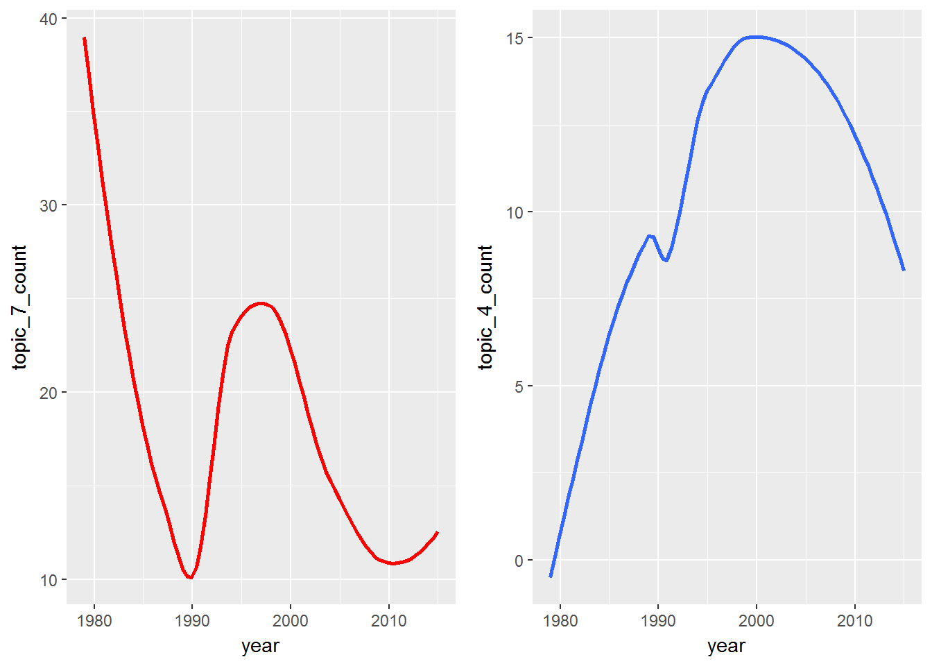
- Themes Over Time
Since the Prince dataset contains year, you can track the themes over time.
You can be really creative here, but for now just look at a few words from two topics and view the frequency over time.
Trending could be an entire tutorial in itself, so if you're really interested, check out this resource.
p1 <- prince_tidy %>%
filter(!year == "NA") %>% #remove songs without years
filter(word %in% c("music", "party", "dance")) %>%
grid.arrange(p1, p2, ncol = 2)
 create your own contribution to the world of AI.
You used data from lyrics and nonfiction books to identify themes, classify individual documents into the most likely topics, and identify similar writers based on thematic content.
Thus you were able to build a simple recommendation system based on text and labeled writers.
Keep in min; you're trying to model art with machines.
An artist could say "You are the apple of my eye", but they are not referring to fruit or body parts.
You have to find what is hidden.
When you listen to music, you don't always hear the background vocals, but they are there.
Turn up your favorite song and listen past the lead vocals and you may be surprised to find a world of hidden information.
So put logic in the background and bring creativity to the forefront during your exploration!
As in all tutorials in this series, I encourage you to use the data presented here as a fun case study, but also as an idea generator for analyzing text that interests you.
It may be your own favorite artists, social media, corporate, scientific, or socio-economic text.
What are your thoughts about potential applications of topic modeling? Please leave a comment below with your ideas!
Stay tuned for Part Three (the fourth article) of this series: Lyric Analysis: Predictive Analytics using Machine Learning with R.
There you will use lyrics and labeled metadata to predict the future of a song.
You'll work with several different algorithms such as Decision Trees, Naive Bayes, and more to predict genre, decade, and possibly even whether or not a song will hit the charts! I hope to see you soon!
Caveats:
Caveat one: The only way you'll get the same results I did is if you run the code in the exact same order with the same, unmodified data files.
Otherwise, reference to specific topics will not make sense.
Caveat two: There are no hard and fast rules on this work, and it is based on my own research.
Although topic modeling does exist in real-world applications, there is not much activity around developing musical recommenders based entirely on lyrics.
Caveat three: Topic modeling is tricky.
Building the model is one thing, but interpreting the results is challenging, subjective, and difficult to validate fully (although research is underway: see this article by Thomas W.
Jones).
The process is unsupervised, generative, iterative, and based on probabilities.
Topics are subtle, hidden and implied and not explicit.
create your own contribution to the world of AI.
You used data from lyrics and nonfiction books to identify themes, classify individual documents into the most likely topics, and identify similar writers based on thematic content.
Thus you were able to build a simple recommendation system based on text and labeled writers.
Keep in min; you're trying to model art with machines.
An artist could say "You are the apple of my eye", but they are not referring to fruit or body parts.
You have to find what is hidden.
When you listen to music, you don't always hear the background vocals, but they are there.
Turn up your favorite song and listen past the lead vocals and you may be surprised to find a world of hidden information.
So put logic in the background and bring creativity to the forefront during your exploration!
As in all tutorials in this series, I encourage you to use the data presented here as a fun case study, but also as an idea generator for analyzing text that interests you.
It may be your own favorite artists, social media, corporate, scientific, or socio-economic text.
What are your thoughts about potential applications of topic modeling? Please leave a comment below with your ideas!
Stay tuned for Part Three (the fourth article) of this series: Lyric Analysis: Predictive Analytics using Machine Learning with R.
There you will use lyrics and labeled metadata to predict the future of a song.
You'll work with several different algorithms such as Decision Trees, Naive Bayes, and more to predict genre, decade, and possibly even whether or not a song will hit the charts! I hope to see you soon!
Caveats:
Caveat one: The only way you'll get the same results I did is if you run the code in the exact same order with the same, unmodified data files.
Otherwise, reference to specific topics will not make sense.
Caveat two: There are no hard and fast rules on this work, and it is based on my own research.
Although topic modeling does exist in real-world applications, there is not much activity around developing musical recommenders based entirely on lyrics.
Caveat three: Topic modeling is tricky.
Building the model is one thing, but interpreting the results is challenging, subjective, and difficult to validate fully (although research is underway: see this article by Thomas W.
Jones).
The process is unsupervised, generative, iterative, and based on probabilities.
Topics are subtle, hidden and implied and not explicit.